Spherical Harmonics and applications in real time graphics

Yikes; it's been awhile since my last update!

I wanted to share a little bit of information from a technique I've recently been working on for an unrelated project. The technique uses a series of equations called "spherical harmonics" for extremely efficient high quality diffuse environment illumination.

This is a technique that started to become popular maybe around 15 years ago -- possibly because of its usefulness on low power hardware. It fell out of favour for awhile, I was never entirely clear why. I got some good value from it back then, and I hope to get more good value from the technique now; so perhaps it's time for spherical harmonic's star to come around again?

There's a fair amount of information about spherical harmonics on the internet, but some of can be a little dense. There seems to be lack of information on how to take the first few steps in applying this math to the graphics domain (for example, for diffuse environment lighting). So I'll try to keep this page approachable for graphics programmers, while also linking off to some of the more dense and abstract stuff later on. And I'll focus specifically on how I'm using this math for graphics, how I've used it in the past, and how I'd like that to grow in the future.

What are spherical harmonics

The "spherical harmonics" are a series of equations that we'll use to compress lighting information greatly. The easiest way to understand them is to start with something simpler and analogous -- and that is cubic splines.

Splines are a method of describing a curve through space with a finite number of points (or points and tangents). Even though the curve is defined by a finite number of parameters, the result is effectively an infinite number of points. To define the curve, we need equations of the form:

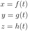
Where t is the distance along the spline (usually between 0 and 1) and x, y & z are cartesian coordinates. In the case of cubic splines, the functions f, h and g are cubic polynomials. If you've used Bezier splines before, you may be familiar with a way to express these polynomials using a form called a "Bernstein polynomial".

Bernstein basis

Imagine the folowing 4 equations:

By Ben FrantzDale (Graphed in Matplotlib.) [GFDL (http://www.gnu.org/copyleft/fdl.html) or CC BY-SA 4.0-3.0-2.5-2.0-1.0 (http://creativecommons.org/licenses/by-sa/4.0-3.0-2.5-2.0-1.0)], via Wikimedia Commons

These are the Bernstein basis functions (B0(), B1(), B2(), B3()). Using these functions, we can express a cubic polynomial in this form:

Where w0, w1, w2 & w3 are constant weights. The four weight values will determine the shape of the curve we get. This is the important thing -- the Bernstein basis functions are defined so that we get any cubic polynomial function, just by changing the 4 weight values. And the four weight values provide a convenient way to express a spline (alternatively we can do similar things with other basis functions -- like the Hermite basis, or for different types of equations, the Fourier basis).

When dealing with cubic polynormals, we use 4 Bernstein basis equations; but the equations are defined for any degree polynomials. So, for example, if we were working with 5th degree polynomials, then we could calculate 6 associated Bernstein basis functions.

SH basis

But we want to know how this relates to spherical harmonics! (But the interested might want to diverge off to Wolfram & Wikipedia: http://mathworld.wolfram.com/BernsteinPolynomial.html, https://en.wikipedia.org/wiki/B%C3%A9zier_curve).

It turns out that the "spherical harmonics" are actually a series of equations which are a little bit similar to the Bernstein basis functions ("harmonic" being just a name for a certain kind of equation). But the spherical harmonics are special because they are defined for a very specific type of data. And that is values that are defined across the surface of a sphere...

Above, we used Bernstein basis functions to express polynomials. But the type of function that can be expressed using spherical harmonics looks a little like this:

Here, theta and phi are spherical coordinates. Also note that another way to express the spherical coordinates theta and phi is by using a unit length vector!

Simplest application in graphics

So why is this type of equation useful? Well, there's another common construct in graphics that represents values stored over the surface of sphere -- that is a cubemap.

When we use a cubemap for the background sky in a shader, we probably have a line of shader code a little like this: float3 skyColor = MySkyCubeMap.Sample(MySampler, unitLengthVector.xyz).rgb;

For any given direction, the cubemap will give us a colour value. Even though it's a cubemap, it's defining colour values across the surface of a sphere (before cubemaps we used other mappings, like spheremaps and paraboloid maps -- but it turns out that, oddly, a cube is just the cheapest approximation to a sphere for shaders). We could use spherical harmonics to do something very similar.

In the spline example, the analogous operation would be fitting a curve to texture values. So imagine we had an RGB single dimensional texture. We would need 1 spline for each component, but let's take red as an example. Since this is a 1D texture, we can graph the red values against the (1D) texture coordinate as so:

In theory, we can find a best fit cubic spline for this data. If we do that, we can use the spline as a (non-discrete) replacement for the texture (if we were doing the reverse -- using a texture as a replacement for a function -- we would called it a lookup table).

The degree of the spline will determine how accurately we can approach the source data. Most textures would need very high degree polynomials to even get close. In general, high frequency information is hard to replicate, but low frequency information can sometimes come through.

In practice, this usually isn't a very useful thing to do -- though there are applications along this line of thought (such as cubic interpolation between texels, particularly with terrain heightmaps). We're also starting to tread on "signal processing" ground (which we might use for deep ocean wave simulations, like the one in XLE).

So why would we ever want to replace a cubemap with a function using spherical harmonics? Isn't that just as useless? The answer is no! There are some important cases where spherical harmonics are both accurate enough and useful enough to be worth our attention!

Cartesian spherical harmonics

The spherical harmonics can be expressed in spherical coordinates or cartesian coordinates. For graphics, the cartesian form is much more useful.

Our notation for the harmonics themselves will be this:

Where l (lower case L) is the "band index" and m is a value with the constraint -l ≤ m ≤ l. The number of bands is the analogue of the degree of a polynomial -- more bands means greater accuracy and better reproduction of higher frequency data. For realtime stuff, we'll focus on the first 3 "bands". If you look around Wolfram or Wikipedia, you'll see more complex forms of the equations. But this form is good for our applications.

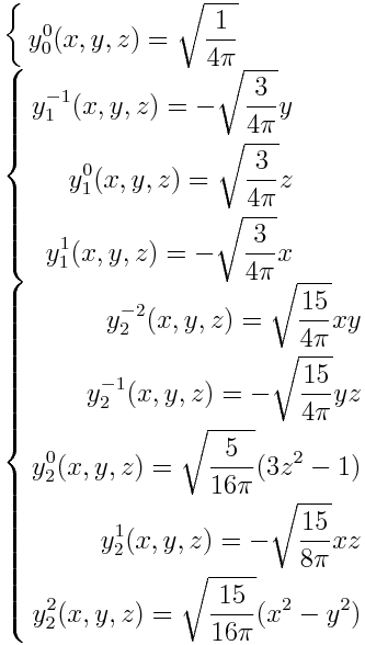
There are the first 3 bands, in the form we'll use in XLE:

To get a sense of how these equations look in 3D space, here's a picture of the first 4 bands from Wikipedia (note that the blue represents positive numbers, the yellow is negative):

By Inigo.quilez (Own work) [CC BY-SA 3.0 (http://creativecommons.org/licenses/by-sa/3.0)], via Wikimedia Commons

It's important to be aware that you'll see slightly different variations of these equations in different publications. This is why it's not always safe to combine equations from different sources (such as the rotation equations and optimization equations we'll get to later).

• this form employs the "Condon-Shortley phase". This basically just adds the negative sign in front of some of the equations. This reduces the complexity of some of derived equations (such as the equations for rotation). Not all graphics literature use this form (for example, Robin Green doesn't, but Peter-Pike Sloan does)
• the order in which y, z & x appear in band 1 can be different in different forms (this ordering seems to be most common, but it does make the rotation code a little more confusing)
• this form assumes that the vector [x y z] is unit length (ie: x^2+y^2+z^2=1). For our applications, that's always true -- but many sources don't mention that as an assumption
• the equation for m=0 & l=2 is often expressed with 2z^2 - x^2 - y^2 in the brackets. But, given the unit length assumption, this equivalent
• finally, there seems to be some uncertainty about the constant in the equation when m=2 & l=2 (maybe?). While working on this page, I noticed that some sources have 15/16, others have 15/32. I'm not sure what' going on there -- I might have to re-derive the equation to figure that out

In short, we can't just copy/paste our why through spherical harmonics. We have to know what's going on. (It's also a good example of why you should never trust the correctness of any code you find on the internet!)

Projecting into spherical harmonics and reconstruction

As mentioned above, we want to combine the spherical harmonics with weight values, and use this combination to express some complex spherical function. Converting a function into spherical harmonics is called "projection." Using the spherical harmonics to get back an approximation of the original function is called "reconstruction."

The projected form of a function is just the set of weights -- one weight for each spherical harmonic (up to some limit on the number of bands). The weights are called coefficients. Let's say our input function is the red channel of a cubemap. We'll use 3 bands to approximate that -- that's 9 equations, and 9 coefficients. Since we also want the green and blue channels, that's another 9 coefficients per channel.

In effect, we end up with an approximation of the input cubemap in just 9 color values. Obviously we can't represent much high frequency data with so few colours. We could get higher quality versions with more bands (4 bands would be 16 colour coefficients, 5 would be 25, 6 would be 36). This might be useful for spherical reflections, but for diffuse (as we'll see later) there's a good reason to stop at 3 bands.

Projection and Reconstruction

Projection is surprising simple. We can calculate each coefficient separately, and we do that by just finding the integral of the input function multiplied by the corresponding spherical harmonic.

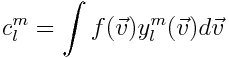
Since our input function is discreet (ie, it's just pixels in a cubemap), the integral becomes simple. We just need to multiply the pixel values by the spherical harmonic for the cubemap direction -- the only difficulty is to weight for the solid angle of the cubemap pixel (see the XLE shader code for this equation).

The reconstruction formula is also very simple; and should now look oddly familiar:

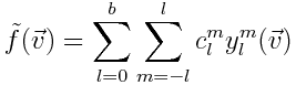
Here, we just take the weighted sum of the spherical harmonics for a given direction (where b is the band number limit). It's pretty straight forward; but it gets more complex from here.

Example

So what does it look like? Here's an example environment texture and the equivalent constructed environment. I'm going to skip ahead just a bit and show how it looks when we construct diffuse reflectance from an environment texture. These are equirectangular panorama maps; trivially compressed to LDR jpgs.

Source texture

(from sIBL Archive: http://www.hdrlabs.com/sibl/archive.html)

Reference diffuse response

ie, for each direction in the panorama map, this shows the correct diffuse response of the environment, from a plain lambert diffuse BRDF.

Reconstructed response with spherical harmonics compression

Absolute difference multiplied by 20

The reconstructed response is using 3 bands; so it's stored using just 9 colour values. As you can see, there is some information loss -- but we can actually prove mathematically that the maximum error is pretty small.

To be continued

So, we've got the very basics down. We know enough to be able to compress a cubemap down to spherical harmonic form, and reconstruct an approximation from that.

Alone, it may sound like an interesting thing to do; but it's not very useful yet. I'll follow this up with some details on how we can use spherical harmonics for some really interesting stuff. Still to cover:

• combining our compressed environment information with the lambert diffuse equation
• building optimized reconstruction code for shaders
• rotating and manipulating spherical harmonics at runtime (and optimization thereof)
• applications in global illumination schemes
• some examples from around the web, and a list of the right literature to follow up with
• some cool examples of SH used in games (eg; The Last of Us, The Order: 1886)!