Spherical Harmonics and applications in real time graphics (part 2)

This is a continuation of the previous page; a tutorial for using spherical harmonic methods for real time graphics. On this page we start to dig into slightly more complex math concepts -- but I'll try to keep it approachable, while still sticking to the correct concepts and terms.

Integrating the diffuse BRDF

On the previous page, we reconstructed a value from a panorama map that was compressed as a spherical harmonic. The result is a blurry version of the original panorama.

Our ultimate goal is much more exciting, though -- what if we could calculate the diffuse reflections at a material should exhibit, if it was placed within that environment?

This is the fundamental goal of "image based" real time lighting methods. The easiest way to think about it is this -- we want to treat every texel of the input texture as a separate light. Each light is a small cone light at an infinite distance. The color texture of texel tells us the color and brightness of the light (and since we're probably using a HDR input texture, we can have a broad range of brightnesses).

Effectively, the input texture represents the "incident" light on an object. We want to calculate the "excident" light -- or the light that reflects off in the direction of the eye. We're making an assumption that the lighting is coming from far away, and the object is small.

Since our input texture has a finite number of texels, we could achieve this with a large linear sum:

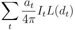
Where t is a texel in the input texture, I is the color in the input texture, d is the direction defined by the mapping (ie, equirectangular or cubemap), a is the solid angle of the texel, and L() is our (somewhat less than bi-directional) BRDF. In spherical harmonic form, we would have to express this equation as a integral (because the spherical harmonic form is a non-discrete function).

But we can do better than this. It might be tempting to consider the blurred spherical harmonic reconstruction of the environment as close enough -- but, again, we can do better!

Zonal harmonics

We've talked about using spherical harmonics to represent data across a sphere. But certain type of data can be expressed in a even more compressed form. For example, if the data has rotational symmetry, we can take advantage of that.

Let's consider a vector dot product:

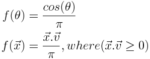
Where u is a constant 3d vector. If the parameter, x, is a unit length 3d vector, then we have an equation that can be represented as a spherical harmonic. However, this equation is rotationally symmetrical around the u axis (meaning we can rotate x around u without changing the value of f(x)).

For convenience, we'll set u to be +Z. Now, only the z component of x has any bearing. As a result, when we build the spherical harmonics for this equation, the harmonics that use the x and y components can be discarded. It turns out that only the harmonics where m = 0 will remain -- that is, we end up with one harmonic per band, and it's the middle one.

So, this convention of preferring +Z as the central axis for equations with rotational symmetry is part of the reason we express the harmonics as they are, in the order that they typically appear (but, as we'll find out, the rotational invariance property means that other conventions would work just as well).

This new set of harmonics (with rotational symmetry around the +Z axis) are called "zonal harmonics." They can be useful for simplifying some operations down to more manageable levels.

BRDF as a zonal harmonic

Obviously, when we say "diffuse BRDF", typically we mean the lambert diffuse equation:

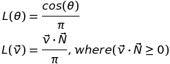
This is one of those cases where the "normalization factor" of 1/pi is important. Sometimes we can ignore that; but here it's critical! (Particularly since we're probably going to combine our diffuse IBL simulation with a specular IBL simulation from the same input texture and we want them to be properly balanced against each other). So, if you're not familiar with it -- better do some research!!

The first we need to do is create a spherical harmonic that represents the BRDF itself (notice that our simple BRDF, with one vector parameter, takes the same form as other equations we've expressed with spherical harmonics -- it, also, is just a function expressed over the surface of a sphere).

For the lambert diffuse, this is straight-forward. We've already seen that we can represent a dot product as a zonal harmonic. All we need to do is modify that for our normalized equation. We can do this by projecting the equation into spherical harmonics (using the formulae in the previous post).

Diffuse SH methods seem to universally use this simple BRDF... But it might be an interesting exercise to extend these ideas for more complex BRDFs. 2 candidates come to mind:

• Oren-Nayar, which introduces a view dependent microfacet simulations
• the Disney diffuse model, which simulates the fresnel effect on both incidence and excidence

But for now, let's just stick with lambert.

Zonal harmonics for lambert diffuse

Here are the resulting coefficients for the first 3 bands (these are derived from Peter-Pike Sloan's "Stupid SH Tricks."):

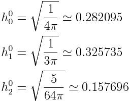
This is a zonal harmonic -- so we only have one coefficient per band. It's also a polynomial approximation of a non-polynomial function, so it can't be perfectly accurate. We should take a look at the consequence of these inaccuracies before we go forward.

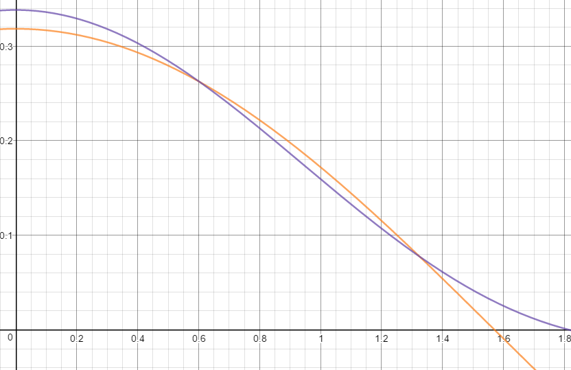
Here, the orange line is cos(theta)/pi and the purple line is our approximation using SH (the x axis is theta). You can find some similar graphs for higher orders in the above reference. As you can see, our approximation seems to drift off a bit, particularly at theta=0 and theta=pi/2.

On the previous page, I showed some images from our final algorithm and another showing the absolute difference from a reference solution multiplied by 30. Here it is again:

The banding suggests that most of the error is coming from high frequency details that are lost to spherical harmonic reconstruction. However, we're also seeing places where bright light appears to be bleeding into dark areas. I wonder if this may be due to the cosine lobe inaccuracies near pi/2.

Convolving our environment by the cosine lobe

Recall the equation we started with:

We can't afford to actually do that sum in real time -- it would mean sampling every pixel in the input texture and multiplying it by the BRDF. We just want some equation that can find the sum in a single step.

Our L() part of this equation represents the zonal harmonic approximation of the BRDF. That's the quantity of reflection for a particular direction. And I represents the spherical harmonic approximation of our environment. That's the amount of incident light from a direction.

We want to find a way to combine these two parts of the equation and evaluate the sum all at once. It turns out, there's a way to do this -- it's called convolution.

That might sound difficult enough, but there's even more to it than that. Our cosine lobe zonal harmonic coefficients are defined only for a normal along +Z. We need a way to rotate the zonal harmonic coefficients relative to the spherical harmonic coefficients (which would be the same as rotating the normal from +Z to some arbitrary direction). We would rotate spherical harmonic coefficients (which we can do arbitrarily and without loss) but actually that formula is fairly expensive. We want something more efficient.

It turns out that there is a way to do all of this at once -- find the convolution and also rotate the zonal harmonic. The equation is oddly simple, and (fortunately for us!) the result is just another set of coefficients, which when added together will give us the final reconstruction.

See Local, Deformable Precomputed Radiance Transfer by Sloan, Luna & Snyder:

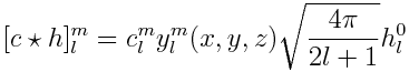
Where h are zonal harmonic coefficients, c are spherical harmonic coefficients, y are the basic SH constants (from the previous page), <x,y,z> is the direction that +Z will be rotated onto, and [c * h] are the convolved output coefficients.

The result (finally) are coefficients that represent the diffuse response, for a given environment, for a given direction. If we summed these coefficients, we would end up with a value that takes into account all incident light, from all directions. And -- to an extraordinarily high accuracy. This works for any environment, and all of this comes from just 9 color coefficients.

This is the equation that makes all of this crazy stuff possible. We've effectively reduced a very complex integral down to a really basic equation. If we didn't have such as simple formula for this convolution and rotation then math might have become unwieldy enough to be unmanageable.

Oddly, though, the role of this equation within the whole SH diffuse mess is frequently not well described in many papers and sources. I've come across a bunch of spherical harmonic implementations that have stumbled in this area, perhaps because it's not very clear. Peter-Pike Sloan talks about it in the above paper, and he references Driscoll and Healy for the derivation... But at that point, that math is getting pretty dense. Other papers (like Ramamoorthi & Hanrahan's seminal paper) tend to deal with it in a somewhat abstract fashion. And in the final shader implemention, the equations will evolve into a completely new form that doesn't look like a convolve at all. So, this step can be easily overlooked.

This is a large part of why I wanted to write this tutorial -- to try to make it a little clearer that there is a critical convolve operation in the middle of this application, and show how that evolves into the constants we'll see later.

Still to come

So; we've figured out how to use spherical harmonics to distill our complex lighting integral down to something manageable and highly compressed.

But there's still a bunch to cover!

• implementing efficient shader code
• rotating arbitrary spherical harmonic coefficients
• cool applications and tricks!