Spherical Harmonics and applications in real time graphics (part 3)
This is a continuation of the tutorial on spherical harmonic applications for games. On the last page, we figured out the core math for integrating a basic diffuse BRDF with a spherical environment of incident light.
Efficient implementation
So far, we've been dealing with spherical harmonics fairly abstractly. But now we can get down to a concrete use and some concrete code. Given our input texture (which effectively describes a sphere of incident light on a point) we want to calculate, for a given normal direction, what is the appropriate diffuse response.
To explain that more visually, here's the images from the first page. The first one is the input texture, and the second one is the matching diffuse response (with the same mapping).
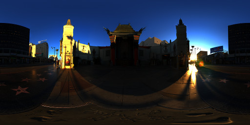

(images from sIBL Archive: http://www.hdrlabs.com/sibl/archive.html)
Recall that we've expressed the BRDF as zonal harmonic coefficients and the incident light environment as spherical harmonic coefficients. We've established that we need to use a "convolve" operation to calculate how the BRDF reflects incident light to excident light (this effectively calculates the integral of the BRDF across the incident sphere). We also worked out that we need to rotate the BRDF in order to align it with the direction of the normal.
To refresh, here's the equation for convolution and rotation:
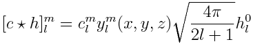
The output of the convolve operation is a set of coefficients, and our final result will be the sum of those coefficients.
Simplifying
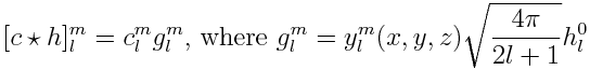
Let's define g by rearranging the convolve equation:
Recall that our coefficients for the cosine lobe zonal harmonic are:
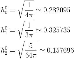
Now, taking the coefficients for the cosine lobe zonal harmonic, we can calculate g for each of the bands.
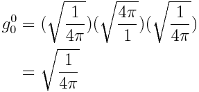
Band 0 (constant):
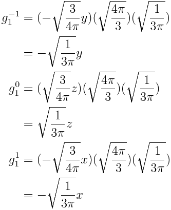
Band 1:
Band 2:
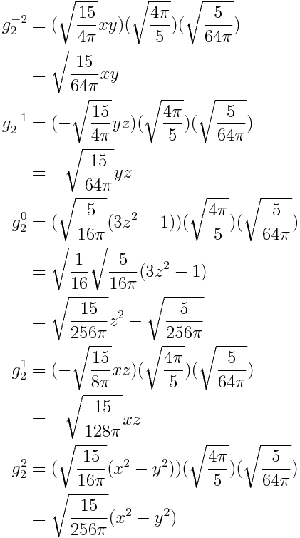
As luck would have it, y() gets almost completely factored out!
Shader implementation tricks
Notice that the g values mostly take the form g = constant * q(x,y,z), where q(x,y,z) is the non-constant part of the appropriate spherical harmonic (eg, x, yz, etc). The first and seventh equations are a bit special -- the first equation is just a constant value and the seventh equation has 2 terms: a constant part and a z^2 term. We can refactor the equations to combine the constant term with the first equation.
To make things a little easier on ourselves, we will pre-multiply the spherical harmonic coefficients by the constant values from the associated g value (taking into account the special case for the seventh one).
That leads us to this modified version of the original reconstruction equation:
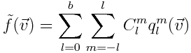
Here, "C" is the "pre-multiplied" coefficient.
We can also decide how to vectorize these calculation. We can think of this operation as the dot product of two 9 dimensional vectors; one vector for the pre-multiplied values, one vector containing the evaluations of q(x,y,z). We also have to do this 3 times (once for each color primary -- red, green and blue).
Some older GPUs had vectorized instructions (or SIMD instructions), which meant that it was more efficient to perform instructions on a full 4D vector, rather than single floats. So there are a few implementations around that use two 4D vectors to do 8 components of the dot product for each color channel (and then add the final constant part).
Modern hardware can keep it's ARUs busy even when just performing single float instructions and as a result, that form of vectorization is less important. Instead, it's often easier for us to just rotate the vectorization around and instead use 8 multiply-add operations with 3 dimensional vectors that just represent the rgb color values. This implementation also doesn't require a dot-product instruction (which, incidentally, was important when implementing this way back on the PS2, where dot products were may difficult due to that hardware's instruction scheduling behaviour).
Final shader
So our final shader implementation turns out to be very basic. XLE uses the second, more straight-forward kind of implementation. We can pre-multiply the "C" constant values on the CPU side (typically either on a per-object basis or a per-scene basis).
float3 ResolveSH_Opt(float3 premulCoefficients[9], float3 dir)
{
    float3 result = premulCoefficients[0];

    result += premulCoefficients[1] * dir.y;
    result += premulCoefficients[2] * dir.z;
    result += premulCoefficients[3] * dir.x;

    float3 dirSq = dir * dir;
    result += premulCoefficients[4] * (dir.x * dir.y);
    result += premulCoefficients[5] * (dir.z * dir.y);
    result += premulCoefficients[6] * dirSq.z;
    result += premulCoefficients[7] * (dir.x * dir.z);
    result += premulCoefficients[8] * (dirSq.x - dirSq.y);
    return result;
}
Recall that the x, y, z inputs to q(x,y,z) are the normal (and it must actually be unit length) -- this is the parameter dir in the above shader. We can choose to evaluate the spherical harmonic on the vertex shader or on the fragment shader. When using normal maps that will typically mean evaluating in the fragment shader.
For lower power hardware, if we have reasonably dense geometry we can evaluate in the vertex shader. This style of lighting is naturally fairly soft and smooth, so linear interpolation across the triangle will often produce reasonable results. But there's one more important detail we haven't discussed: the normal must be in the same coordinate space as the evaluated spherical harmonic coefficients! So does this mean we must transform the normal into world space and do all calculations in that space? That's an option, but as we'll see, there's another way as well.
Rotation
One of the key properties of systems like this that use the spherical harmonics is that they are rotationally invariant. If means that if we can rotate our diffuse reflection approximation (and we can), then we will not loose any precision. Imagine an environment with a bright white light in the +Z direction. If we rotate the environment so that light is in another direction (let's say, +X), then we want the shape and brightness of the light to remain exactly the same. "Rotationally invariant" means that this will be the case regardless of how we rotate the environment. Even though the spherical harmonics appear to use x, y & z differentially, there is no actual bias for any direction (this may be clearer to see in the polar coordinate versions of the harmonics).
To rotate a spherical harmonic lighting environment, we must take each band one-at-time. Band 0 is just a constant, so it requires no rotation. In band 1 (which is 3 components), the equation is actually just a permutation of the basic 3x3 rotation matrix operation (which should make intuitive sense, given the directional parts in the band 1 are just x, y, z). For the band 2 and beyond, we need something more involved.
Rotating the band 2
There is a general formula for rotating spherical harmonics coefficients of an arbitrary band. We'll use this to handle band 2.
In "Spherical Harmonic Lighting: The Gritty Details", Appendix 1, Robin Green describes the basic method we'll be using, which is derived from work by Josepth Ivanic and Klaus Ruedenberg. We have to make some changes to the math, however -- are a couple of import modifications we need to make. First, Robin Green isn't using the Condon-Shortley phase (described in the first part), but we are. Second, there's a small errata in the V matrix.
We'll start by defining six 5x5 matrices: u, v, w and U, V, W. The elements of the final rotation matrix, M will be constructed from these matrices in this way:

The elements of u, v and w are dependent only on l (the band index) m and n. In other words, u, v and w are all constant for band 2. The elements of U, V and W are dependent on the rotation matrix for the previous band (ie, the permutated rotation matrix we used for band 1).
Robin Green shows the definition of these matrices, but given the notes above and since it is a lot of abstract maths, I won't duplicate it here. Instead I'll give some code.
(BTW, as a side note, if you look closely at the definitions for these matrices, you'll see cases that can result in a divide by zero. In these cases, the element on the complementary matrix is zero.)
const int l=2;
Mat5x5 P[3];
memset(&P, 0, sizeof(P));       // (i==-l && l==l rows not filled in by the below loop)
for (int i=-1; i<=1; ++i) {
    for (int a=-1; a<=1; ++a) {
        for (int b=-l; b<=l; ++b) {
            float& dst = P[i+1][a+l][b+l];
            if (b==l) {
                dst =   band1Rotation[i+1][2] * band1Rotation[a+1][ l-1+1]
                    -   band1Rotation[i+1][0] * band1Rotation[a+1][-l+1+1];
            } else if (b==-l) {
                dst =   band1Rotation[i+1][2] * band1Rotation[a+1][-l+1+1]
                    +   band1Rotation[i+1][0] * band1Rotation[a+1][ l-1+1];
            } else {
                dst =   band1Rotation[i+1][1] * band1Rotation[a+1][b+1];
            }
        }
    }
}

Mat5x5 uMat, vMat, wMat;
Mat5x5 UMat, VMat, WMat;
for (int m=-l; m<=l; ++m) {
    for (int n=-l; n<=l; ++n) {
        auto kroneckerDeltam0 = (m==0) ? 1 : 0;
        auto absm = abs(m);
        float d = (n==-l || n==l) ? (2*l*(2*l-1)) : (l+n)*(l-n);
        uMat[m+l][n+l] =        sqrtf(float((l+m)*(l-m))/d);
        vMat[m+l][n+l] =  .5f * sqrtf(float((1+kroneckerDeltam0)*(l+absm-1)*(l+absm))/d) * float(1-2*kroneckerDeltam0);
        wMat[m+l][n+l] = -.5f * sqrtf(float((l-absm-1)*(l-absm))/d) * float(1-kroneckerDeltam0);

        // note --  wMat[m+l][n+l] will be zero if (m == l-1) || (m == l) || (m == 0)
        //          In these cases, the associated 'W' value is undefined -- so we avoid calculating it in those cases
        //          For band 2, this is always the case! Since 'w' is always zero, we also never
        //          actually need to calculate 'W'

        auto kroneckerDeltam1    = (m== 1) ? 1 : 0;
        auto kroneckerDeltamneg1 = (m==-1) ? 1 : 0;
        float& U = UMat[m+l][n+l];
        float& V = VMat[m+l][n+l];
        float& W = WMat[m+l][n+l];
        U = P[ 0+1][   m+l][n+l];
        assert((n+l) >= 0 && (n+l) < 5);
        if (m==0) {
            V = P[ 1+1][   1+l][n+l] + P[-1+1][  -1+l][n+l];
            W = P[ 1+1][ m+1+l][n+l] + P[-1+1][-m-1+l][n+l];        // redundant, but no danger of an out-of-bound matrix access in this case
        } else if (m>0) {
            V = P[ 1+1][ m-1+l][n+l] * sqrtf(float(1+kroneckerDeltam1))
              - P[-1+1][-m+1+l][n+l] * float(1-kroneckerDeltam1);
            if (wMat[m+l][n+l] != 0.f) {
                assert(isValidA(m+1, l) && isValidA(-m-1, l));
                W = P[ 1+1][ m+1+l][n+l] + P[-1+1][-m-1+l][n+l];
            } else {
                W = 0.f;        // (always the case)
            }
        } else if (m<0) {
            V = P[ 1+1][ m+1+l][n+l] * float(1-kroneckerDeltamneg1)
              + P[-1+1][-m-1+l][n+l] * sqrtf(float(1+kroneckerDeltamneg1));         // (Google)
            if (wMat[m+l][n+l] != 0.f) {
                W = P[ 1+1][ m-1+l][n+l] - P[-1+1][-m+1+l][n+l];
            } else {
                W = 0.f;        // (always the case)
            }
        }
    }
}
This code has been thoroughly tested, and is reliable. But since this algorithm seems to have been copied out incorrectly in a number of places, I'll also point out a few other identical implementations:
- in MATLAB code
- also MATLAB
- C++ (but beware errors in other parts of this source file)
Evaluation in local space
Rotating a spherical harmonic coefficient vector allows us to do the shader evaluation in any coordinate space we choose. In some cases, it may be convenient to do the evaluation in the local coordinate space for an object. This is now possible, we just rotate the spherical harmonic coefficients by the inverse of the rotation part of the local-to-world transform (ie, thereby transforming the spherical harmonic coefficients into the object's local space).
This is an interesting advantage of spherical harmonics over cubemaps. Because we're defining our environment mathematically and continuously, they can be a little more malleable.
Practical rotation
The above method is a great reference method for rotating band 2. But it's not very practical in real-world cases. We want something that is at least efficient enough to be done once per object. In an ideal world (as we may see later), we want to be able to do it at a much more granular level. But to do this, we need something far more efficient!
There are a number of different approaches to optimizing rotations. Some methods introduce some errors, others are accurate. But we break them down into 3 broad categories:
- factoring arbitrary rotations into rotations around cardinal axes
- replacing the expensive parts of the algorithm, with cheap approximations
- algebraically refactoring the full rotation algorithm into a form that is specific to band 2 and well suited to our hardware
I'm going to talk about a few of the alternatives, before finally explaining the method I've been using.
Efficient rotation through cardinal rotations
The rotation matrix method above can calculate a transformation matrix for any arbitrary rotation. But it turns out that for some rotations (particularly rotations around the cardinal axes), many elements of the matrix are zero. Furthermore, in the case of rotations around the Z axis, even the non-zero elements are very easy to calculate.
In fact, rotation around the Z axis just follow this template:
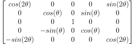
This can actually help us generate a full rotation matrix for an arbitrary rotation. Recall that it's possible to decompose any 3D rotation into Euler angle form. In this form, the rotation is described by 3 angles, and each angle is a rotation around a cardinal axis. For example, a rotation in "XYZ" Euler angles form would be 3 angles, one representing a rotation around the X axis, another for a rotation around the Y axis and another for a rotation around the Z axis.
There are many different forms of Euler angles, but the form we're going to use is "ZYZ" form. In this form, there are 2 rotations around the Z axis; but due to the rotation around the Y axis in the middle, the second Z axis is enough to provide the third degree of freedom we need.
Clearly this is convenient because we can just use the simple template above to build the rotation matrices for the two rotations about the Z direction. After we also build the rotation matrix for the rotation around Y, we will just multiply those 3 rotation matrices together.
But how to generate a rotation around the Y axis? Unfortunately, rotations around the Y axis don't come out as cleanly as rotations around the Z axis. But we can use another trick. We can rotate the entire coordinate space to align the Y axis with the Z axis. Then we just rotate around the Z axis again, and rotate coordinate space back.
Aligning Y with Z requires a 90 degree rotation around the X axis (though it may depend on the handiness of your coordinate system). This method actually ends up requiring us to multiply together 5 rotation matrices. 3 of those are rotations around Z, and the remaining 2 are constant matrices.
This method is called "ZXZXZ" (referencing the 3 Z rotations and the two "aligning" X axis rotations). It was first proposed by Kautz, Sloan and Synder in Fast, Arbitrary BRDF Shading for Low-Frequency Lighting Using Spherical Harmonics (hidden away in the appendix).
Substituting approximations
The ZXZXZ method give us accurate results, but the 2 extra matrix multiplies added by the "XZX" step are still frustrating. It would be much nicer if we could just generate an arbitrary rotation around X or Y directly.
Sometimes it can be profitable to simplify a complex equation using a standard approximation technique, such as a Taylor series. This has been proposed as solution to our problem by Jaroslav Krivanek, Jaakko Konttinen, Sumanta Pattanaik and Kadi Bouatouch in "Fast Approximation to Spherical Harmonic Rotation".
Their goal is to rotate coefficient vectors for higher order bands (eg, 5+ bands) that represent specular response. This makes it view-dependent, which requires rotating once per fragment shader (as opposed to once per object, as in our diffuse methods).
They found that their method was accurate for rotations less than 20 degrees for their Phong lobe (but keep in mind this only applies to the Y rotation part, the two Z rotations are still accurate). Obviously that level of accuracy is only useful for very specific solutions.
The equations they are attempting to approximate don't seem to be well suited to Taylor series. But I wonder if this approach could be improved by adjusting the parameterization.
Factoring into zonal harmonics
Derek Nowrouzezahrai, Patricio Simari and Eugene Fiume describe a method in "Sparse Zonal Harmonic Factorization for Efficient SH Rotation" that involves decomposing an SH coefficient vector into a number of zonal harmonics coefficients with fixed rotations. They found that the coefficients for band l of an arbitrary SH could be represented by a sum of at most 2l + 1 oriented zonal harmonic coefficients. This leads to a method for rotation that can be more efficient than ZXZXZ, while still being perfectly accurate.
In this method they have some freedom as to pick the orientations for the zonal harmonic coefficients. They describe a technique that attempts to minimize the number of zonal harmonic coefficients required, thereby also reducing the rotation cost. It's not exactly trivial, but it's a very interesting approach.
You can still find a demo of this technique being used for realtime global illumination in WebGL!
Still to come
So, on this page we covered a lot of stuff -- we wrote the first little bit of shader code, looked at the algorithm for rotating a spherical harmonics coefficient vector, and started explore some methods for optimizing rotations. But there's still a lot to cover! The methods here for rotating efficiently are interesting, but as we'll see, there are better options for our applications.
Also to come -- how to apply spherical harmonics to more than just the diffuse reflections we've been talking about so far.
blog comments powered by Disqus