Improved IBL

I've been working on improving the accuracy of the Imaged Based Lighting (IBL) solution for XLE. This is the technology that allows us to load in a background panorama map and use it for both diffuse and specular lighting.

The best way to do this is by comparing our real-time result to other renderers. So, for example, I've been experimenting with Substance Designer (more on that later). It has nVidia's "IRay" raytracer built-in -- so we can compare the non-real-time results from IRay with real-time XLE. I have other ways to do this, also -- for example, the shader in ToolsHelper/BRDFSlice.sh can generate textures directly comparable with Disney's BRDFExplorer tool.

While doing this (and working on the specular transmission stuff), I've found some interesting improvements to the IBL solution!

Conclusion

This is a really long post; so I'll start with the conclusion. I've made a number of improvements that make the IBL solution appear more realistic, and more similar to ray tracers.

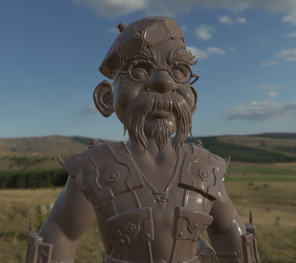"Jamie Gnome" model from here: http://www.turbosquid.com/3d-models/free-obj-mode-jamie-hyneman-gnome/789391

I found some errors in some source material I referenced and fixed some incorrect assumptions I made. Each change is small. But when added up, they make a big difference. The IBL specular is has a lot much punch, things are jumping off the screen better.

Now, I'll go into detail about what's changed.

IBL basis

I've been using a split-term style IBL solution, as per Brian Karis' Siggraph 2013 course (see http://blog.selfshadow.com/publications/s2013-shading-course/). As far as I know, this is the same method used in Unreal (though I haven't checked that, there may have been some changes since 2013).

This splits the IBL equation into two separate equations. In one equation, we calculate the reflected light from a uniform white environment. In a sense, this is calculating our reflective a given pixel is, with equal weighting to each direction. Our solution has to make some simplifications to the BRDF (to reduce the number of variables), but we use most of it.

Microfacets!

We can think about this on a microfacet level. Remember our specular equation is an approximate simulation of the microfacet detail of a surface.

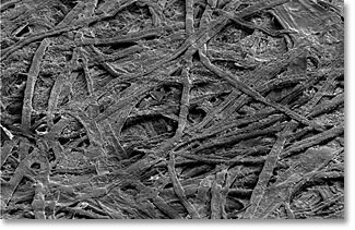
This is a microscopic photo by Gang Xiong, Durham University. It shows a smooth plastic surface.

Each microscopic surface has a normal -- this is the microfacet normal. Remember that "D" represents how the microfacet normal are distributed, relative to the surface normal. For example, in very smooth surfaces, microfacet normals are more likely to be close to the surface normal. This is the most important part of the equation in terms of the actual shape of highlights.

The "G" term is for microscopic scale shadowing between different microfacets. This is why G is close to 1 for most of the range and drops off to zero around the edges. It "fights" the F term, and prevents excessive halos around the edges of things.

And "F" is for the fresnel effect, which determines how much incident light is actually reflected at a given angle. In the specular equation, we're calculating the fresnel effect on a microfacet level, not on the level of the surface normal.

A little bit of history

Most of this stuff actually dates back to 1967 with Torrance & Sparrow. It evolved up to around 1981 with Cook & Torrance (yes, same Torrance). But then nothing much happened for awhile. Then Walter, et al., rediscovered some old math in 2007 (and introduced the term, GGX). And we kind of discovered everything we were doing between 1981 and 2007 was a little bit wrong.

More recently, Brent Burley and Disney found a novel way to visualize multi-parameter BRDFs in a 2D image. They used this to compare our equations to real world surfaces. And so now we have a clearer idea of what's really working and not working.

Anyway, that's why specular highlights in PS4 games feel much "brighter" than previous generations. The shape of the highlight greatly affects the impression of brightness.

There's a great picture here:

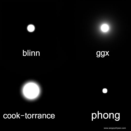
The "GGX" dot is not any brighter... But it appears to glow because of the shape of the falloff.

Second split term part

Anyway, the second part of the split term equation is the environment texture itself. In XLE, this is a cubemap.

Each microfacet will reflect a slightly different part of the image. And our specular equation (D, G & F) effect the brightness of that particular reflection.

However, in this approximation, we only know the average effect of all microfacets, and we can only afford to take a single sample of this cubemap. So, we want to pre-blur the cubemap to most closely approximate the results if we had sampled every microfacet separately.

In XLE, we can use the cvar "cv.IBLRef = true" to enable a "reference" specular equation that samples many evenly distributed microfacets. We want to try to match that.

Sampling microfacets

Since our reflection simulation is based on the microfacet normal, in order to calculate the specular for a pixel, we want to know what microfacets there are in that pixel. But that's far too difficult. We can simplify it down a little bit. What we do know is the probability for the angle between the microfacet normal and the surface normal. This is the "D" term.

For our pre-calculation steps, we sometimes need an accurate sample for a pixel. To do this, we can generate random microfacet normals, and use the D term to weight the effect of each microfacet normal. A little more on this later...

Blurring convolution

What is the ideal convolution to use? Brian Karis suggests a simple convolution involving N dot L. Previously, I was using a method suggested by another project that weights the textures by the entire specular equation. So what is the best method to use?

The blurring method is actually a little similar to the reference specular equation. For every direction in the cubemap, we imagine a parallel flat surface that is reflecting that point. For roughness=0, we should get a perfectly clear reflection. As the roughness value increases, our surface should become more and more blurry. The result is actually only current for surfaces that are parallel to what they are reflecting. On the edges, the reflection should stretch out -- but this phenomenon doesn't occur in our approximation. In practice, this is not a major issue.

The roughness value affects the microfacet distribution and this is what leads to the blurriness. So, we can generate a random set of microfacets, weight them by "D" and then find the average of those normals. That should cause the blurriness to vary against roughness correctly.

But is there better filtering than that? What is the ideal "weight" value for each microfacet normal?

Our goals for filtering should be twofold:

1. Try to replicate the "GGX" falloff shape. A bright pixel in the reflection should appear the same as a dynamically calculated specular highlight. The GGX falloff is also just nice, visually. So we want the falloff to match closely.
2. Try to prevent sampling errors. This can occur when low probability samples are weighted too highly.

I played around with this for awhile and eventually decided that there is a simple, intuitive answer to this equation.

In our simple case where the surface is parallel to the reflection, when we sample the final blurred cubemap, we will be sampling in the direction of the normal. We're actually trying to calculate the effect of the microfacets on this reflection. So, why don't we just weight the microfacet normal by the ratio of the specular for the microfacet normal to the specular for the surface normal?

Since the specular for the normal is constant over all samples, that factors out. And the final weighting is just the specular equation for that microfacet normal (what I mean is, we use the sampled microfacet normal as the "half-vector", or M, in the full specular equation).

This weighting gives us the GGX shape (because it is GGX). It also makes sense intuitively. So, in the end the best method was actually what I originally had. But now the code & the reasons are a little clearer.

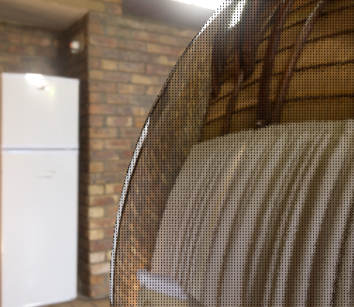
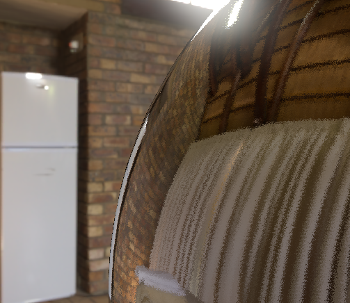
Example

Here is an example of a filtered specular map:

Original image from sIBL archive: http://www.hdrlabs.com/sibl/archive.html

Notice that bright point still appears bright as they are filtered down. They are retaining the GGX shape. Also, when there are bright points, the light energy from those points will get spread out in lower mipmaps. So the bright points become successively wider but darker.

Currently, we have a linear mapping from roughness -> mipmap. But as you can see, often we have more resolution that we actually need. So we could change this to a non-linear mapping.

Sampling errors

At high roughness values, we can get some sampling errors. In HDR environment textures, some pixels can be hundreds or thousands of times brighter than the average pixel. As a result, these pixels overwhelm hundreds or thousands of other pixels. Our sampling pattern attempts to cluster more samples in more areas. If a pixel like this is picked up in an "unimportant" area, where are are few samples, they can lead to artifacts.

The following mip chain was generated from an image where the point in a middle of the sun is so bright that it can't be represented as a 16-bit float. This causes errors, and you can see how the errors radiate outwards according to the sampling pattern.

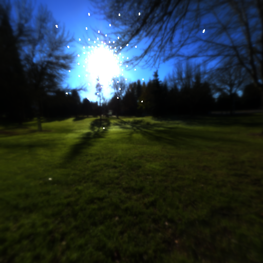
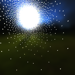
Original image CC-Zero from http://giantcowfilms.com/.

This particular case can only be solved by a better float32 -> float16 converter than clamps values against the valid range. But it's a good way to visualize how a few pixels can affect many other pixels.

It may be possible to get improvements by sampling every input pixel for every output pixel. This might not be such a bad idea, so if I get a chance, I'll try it.

There's also another possible sampling improvement related to the "G" term. Using the microfacet normal rather than the surface normal could help reduce the effect of samples around the extreme edge of the sampling pattern. See "M vs N in G" below for more details on that.

Improved microfacet sampling

When we build the set of random microfacets, we don't necessarily have to distribute those microfacets evenly. We want some "important" microfacets to be more likely, and "unimportant" microfacets to be less likely.

Previously, I was using the sampling pattern suggested by Karis in his course notes. However, it's possible that there is an error in that equation.

I've gone back to the original microfacet distribution function by Walter in "Microfacet Models for Refraction through Rough Surfaces" (the GGX paper). He built this pattern specifically for GGX, and he also designed it for both reflection and transmission. This means the view direction isn't considered in the distribution (which is great for us).

Karis' function for generating the microfacet direction actually agrees with this paper (though it is in an optimized form). However, there is a difference in the "Probability Density Functions" (or PDFs) for both:

1. Karis' PDF is (D * NdotH) / (4.f * VdotH)
2. Walter's PDF is D * NdotH

Here, Karis' PDF seems immediately suspicious because the view direction is a factor in the PDF, but not a factor in the microfacet function itself. That seems odd. The factor of "4" is also and area of confusion, because it appears in some versions of the Cook-Torrance microfacet equations, but not others. It's not clear why Karis included it, but it may be because he is using a different form of the Cook-Torrance equation to XLE?

When I switched to Walter's sampling equations, I found 2 immediate improvements:

Floating point errors in microfacet function

Karis' microfacet distribution function is not working perfectly, possibly because of floating point errors (or weird edge cases). I've replaced his equation with another equation that is mathematically identically, but I get much better results.

Sometimes the shader compiler's optimizations can change the mathematics to a point where is it visibly wrong. Could this be the case here?

Old equation:

New equation

They should be producing the same results, but the old version appears to be producing incorrect results for inputs within a certain range. The inputs are "dithered" according to a 4x4 pattern in this example, which is why is appears regular.

Edges are too dark

The differences in the PDF equation are actually making the edges too dark. This is related to the VdotH term. It makes sense to remove VdotH from the PDF for two reasons:

1. The view direction has no impact on the microfacets generated
2. We want to use this sampling in view independent equations

Old version:

New version:

In the new version, the extreme edges are much brighter. The dark halo we get with the old version seems unnatural & incorrect.

NdotL

I've added the NdotL term into IBL, as well. This was previously excluded but is required to match our dynamic specular equation.

This is visually important -- without it, the edges become excessively bright, brighter than the thing they are reflecting. With NdotL, the brightness correctly matches the reflected object.

In effect, we've removed a VdotH term, and added a NdotL. Note that VdotH is the same as LdotH when the "H" is the half-vector between L and V... So this might be source for the mysterious VdotH term in Karis' PDF! He may have assumed that this was part of the PDF, when in fact he was just compensating for a part of his specular equation. If that's the case, though, why isn't it explained in his course notes?

Rebuilding the lookup table

Our split-term solution involves a texture lookup table "glosslut.dds." This is built from all of the math on this page. Our previous version was very similar to Karis' version. But let's rebuild it, and see what happens!

Old version:

New version:

So, the changes are subtle, but important. The specular is general a little bit darker, except at the edges of objects where it has become significantly brighter.

Comparisons

Old look up table:

New look up table:

Reference:

This is just changing the lookup-table. You can see how the reflection is slightly darker in the new version, except that the edges are much brighter. Also, new version matches our reference image much better.

At high F0 values (and along the edges) the reflection appears to be the correct brightness to match the environment.

Alpha remapping

One thing to note is that in XLE, the same alpha remapping is used for IBL that is used for dynamic specular maps. Karis suggests using different remapping for IBL, explaining that the normal remapping produces edges that are too dark. It seems like we've discovered the true cause of the dark edges and the results seem to look fine for us with our normal remapping.

Also, since we're using the exact same specular equation as we use for dynamic lighting, the two will also match well.

Diffuse normalization

Previously, I had been assuming our texture pipeline had was premultiplying the "1/pi" diffuse normalization factor into the diffuse IBL texture. However, that turned out to be incorrect. I've compensated for now by adding this term into the shader. However, I would be ideal if we could take care of this during the texture processing step.

With this change (and the changes to specular brightness), the diffuse and specular are better matched. This is particularly important for surfaces that are partially metal and partially dielectric -- because the diffuse on the dielectric part must feel matched when compared to the specular on the metal part.

Further research

Here are some more ideal for further improvements.

H vs N in G calculation

There is an interesting problem related to the use of the normal in the "G" part of the specular equation. Different sources actually feed different dot products into this equation:

1. Some use N dot L and N dot V
2. Others use H dot L and H dot V (where H is the half-vector or microfacet normal)

For our dynamic specular lights, we are using a single value for N and H, so the difference should be very subtle. But when sampling multiple microfacets, we are using many different values for H, with a constant N.

For example, when using the specular equation as a weight while filtering the cubemap, N dot L and N dot V are constant. So they will have no effect on the filtering.

Remember that "G" is the shadowing term. It drops off to zero around the extreme edges. So by using H dot L and H dot V, we could help reduce the effect of extreme samples.

Also, when building the split-term lookup table, N dot V is constant. So it has very little effect. It would be interesting experimenting with the other form in these cases.

On the other hand, in the dynamic specular equation H dot L and H dot V should be equal and very rarely low numbers. So, in that case, it may not make sense to use the half-vector.

Problems when NdotV is < .15f

Rough objects current tend to have a few pixels around the edges that have no reflection. It's isn't really visible in the dielectric case. But with metals (where there is no diffuse) it shows up as black and looks very strange.

The problem is related to how we're sampling the microfacet normals. As you can imagine, when normals are near perpendicular to view direction, sometimes the microfacet normal will end up pointing away from the view direction. When this happens, we can reject the sample (or calculate some value close to black). When the number of samples rejected is too high, we will end up with a result that is not accurate.

This tends to only affect a few pixels, but it's enough to pop out. We need some better solution around these edge parts.